
Binius STARKs Analysis and Its Optimization
1. Introduction
Distinguished from elliptic curve-based SNARKs, STARKs can be viewed as hash-based SNARKs. One of the main challenges contributing to the current inefficiency of STARKs is that most values in actual programs are relatively small, such as indices in for loops, boolean values, and counters. However, to ensure the security of Merkle tree-based proofs, Reed-Solomon encoding is used to extend data, resulting in many redundant values occupying the entire field, even when the original values themselves are small. Addressing this inefficiency, reducing the field size has become a key strategy.
As shown in Table 1, the first generation of STARKs had a coding width of 252 bits, the second generation 64 bits, and the third generation 32 bits. Despite the reduced coding width in the third generation, there remains significant wasted space. In contrast, binary fields allow for direct bit-level manipulation, enabling compact and efficient encoding with minimal waste. This efficiency is realized in the fourth generation of STARKs.
| STARKs | Base Field | Base Field Width | Coding Efficiency (the higher the better) |
Field Extensions | Typical Projects |
|---|---|---|---|---|---|
| Gen 1 | $p=2^{251}+17 \cdot 2^{192}+1$ | 252 bits | 1 | - | Stone |
| Gen 2 | $p=2^{64}-2^{32}+1$ | 64 bits | 2 | Field Extension 2 | Plonky2, Polygon zkEVM, zkSync zkEVM |
| Gen 3 | $p=2^{31}-2^{27}+1$ | 32 bits | 3 | Field Extension 4 | RISC Zero |
| $p=2^{31}-1$ | 32 bits | 3 | Field Extension 4 | Plonky3, Stwo | |
| Gen 4 | $p=1$ | 1 bit | 4 | Field Extension 128 | Binius |
In comparison to finite fields such as Goldilocks, BabyBear, and Mersenne31, which have gained attention recently, binary field research dates back to the 1980s. Today, binary fields are widely used in cryptography, with notable examples including:
- Advanced Encryption Standard (AES), based on the $\mathbb{F}_{2^8}$ field;
- Galois Message Authentication Code (GMAC), based on the $\mathbb{F}_{2^{128}}$ field;
- QR codes, which utilize Reed-Solomon encoding based on the $\mathbb{F}_{2^8}$ field;
- The original FRI and zk-STARK protocols, as well as the Grøstl hash function, a finalist in the SHA-3 competition, which is based on the $\mathbb{F}_{2^8}$ field and is well-suited for recursive hash algorithms.
When smaller fields are used, field extension operations become increasingly important for ensuring security. The binary field used by Binius relies entirely on field extension to guarantee both security and practical usability. Most of the polynomial computations involved in Prover operations do not need to enter the extended field, as they only need to operate in the base field, thereby achieving high efficiency in the small field. However, random point checks and FRI computations must still be performed in a larger extended field to ensure the necessary level of security.
There are two practical challenges when constructing a proof system based on binary fields: First, the field size used for trace representation in STARKs should be larger than the degree of the polynomial. Second, the field size used for the Merkle tree commitment in STARKs must be greater than the size after Reed-Solomon encoding extension.
Binius is an innovative solution to address these two problems by representing the same data in two different ways: First, by using multivariate (specifically multilinear) polynomials instead of univariate polynomials, representing the entire computation trace through their evaluations over “hypercubes.” Second, since each dimension of the hypercube has a length of 2, it is not possible to perform standard Reed-Solomon extensions like in STARKs, but the hypercube can be treated as a square, and a Reed-Solomon extension can be performed based on this square. This method not only ensures security but also greatly enhances encoding efficiency and computational performance.
2. Binius Principles
The construction of most modern SNARK systems typically consists of the following two components:
- Information-Theoretic Polynomial Interactive Oracle Proof (PIOP): As the core of the proof system, PIOP transforms computational relations from the input into verifiable polynomial equations. Different PIOP protocols allow the prover to send polynomials incrementally through interactions with the verifier. This enables the verifier to confirm the correctness of a computation by querying only a small number of polynomial evaluations. Various PIOP protocols, such as PLONK PIOP, Spartan PIOP, and HyperPlonk PIOP, handle polynomial expressions differently, impacting the performance and efficiency of the overall SNARK system.
- Polynomial Commitment Scheme (PCS): The PCS is a cryptographic tool used to prove that the polynomial equations generated by the PIOP are valid. It allows the prover to commit to a polynomial and verify its evaluations without revealing additional information about the polynomial. Common PCS schemes include KZG, Bulletproofs, FRI (Fast Reed-Solomon IOPP), and Brakedown, each offering distinct performance characteristics, security guarantees, and applicable scenarios.
By selecting different PIOPs and PCS schemes, and combining them with suitable finite fields or elliptic curves, one can construct proof systems with distinct properties. For example:
- Halo2: Combines PLONK PIOP with Bulletproofs PCS and operates on the Pasta curve. Halo2 is designed with scalability in mind and eliminates the trusted setup previously used in the ZCash protocol.
- Plonky2: Combines PLONK PIOP with FRI PCS and is based on the Goldilocks field. Plonky2 is optimized for efficient recursion.
When designing these systems, the compatibility between the chosen PIOP, PCS, and finite field or elliptic curve is critical to ensuring correctness, performance, and security. These combinations influence the size of the SNARK proof, the efficiency of verification, and determine whether the system can achieve transparency without a trusted setup, as well as support advanced features like recursive proofs or proof aggregation.
Binius combines HyperPlonk PIOP with Brakedown PCS and operates in a binary field. Specifically, Binius incorporates five key technologies to achieve both efficiency and security:
- Arithmetic based on towers of binary fields: This forms the computational foundation of Binius, allowing for simplified operations within the binary field.
- HyperPlonk product and permutation checks: Binius adapts HyperPlonk’s product and permutation checks in its PIOP to ensure secure and efficient consistency between variables and their permutations.
- New multilinear shift argument: This optimization improves the verification of multilinear relationships within small fields, enhancing overall efficiency.
- Improved Lasso lookup argument: The protocol incorporates a more flexible and secure lookup mechanism with this advanced argument.
- Small-Field Polynomial Commitment Scheme (PCS): Binius employs a PCS tailored for small fields, reducing the overhead commonly associated with larger fields and enabling an efficient proof system in the binary field.
These innovations enable Binius to offer a compact, high-performance SNARK system, optimized for binary fields while maintaining robust security and scalability.
2.1 Finite Fields: Arithmetic Based on Towers of Binary Fields
Towers of binary fields play a critical role in achieving fast, verifiable computations due to two primary factors: efficient computation and efficient arithmetization. Binary fields inherently support highly efficient arithmetic operations, making them ideal for cryptographic applications sensitive to performance. Moreover, their structure enables a simplified arithmetization process, where operations performed in binary fields can be represented in compact and easily verifiable algebraic forms. These characteristics, combined with the hierarchical structure of towers of binary fields, make them particularly suitable for scalable proof systems like Binius.
| Prime Field$\mathbb{F}_p$ | Binary Field$\mathbb{F}_{2^k}$ | |
|---|---|---|
| Representation | Not canonical | Canonical |
| Addition | Modular Add | Bitwise XOR |
| Multiplication | Modular Mul | No-carry Mul |
The term “canonical” refers to the unique and direct representation of elements in a binary field. For example, in the most basic binary field $\mathbb{F}2$ , any k-bit string can be directly mapped to a k-bit binary field element. This differs from prime fields, which do not offer such a canonical representation within a given number of bits. Although a 32-bit prime field can fit within 32 bits, not every 32-bit string can uniquely correspond to a field element, whereas binary fields provide this one-to-one mapping. In prime fields $\mathbb{F}_p$ , common reduction methods include Barrett reduction , Montgomery reduction , as well as specialized reduction methods for certain finite fields like Mersenne-31 or Goldilocks-64 . In binary fields $\mathbb{F}{2^k}$ , common reduction methods include special reduction (as used in AES), Montgomery reduction (as used in POLYVAL), and recursive reduction (as used in Tower fields). The paper Exploring the Design Space of Prime Field vs. Binary Field ECC-Hardware Implementations notes that binary fields do not require carry propagation in addition or multiplication, and squaring in binary fields is highly efficient due to the simplification rule $(X + Y)^2 = X^2 + Y^2$ .
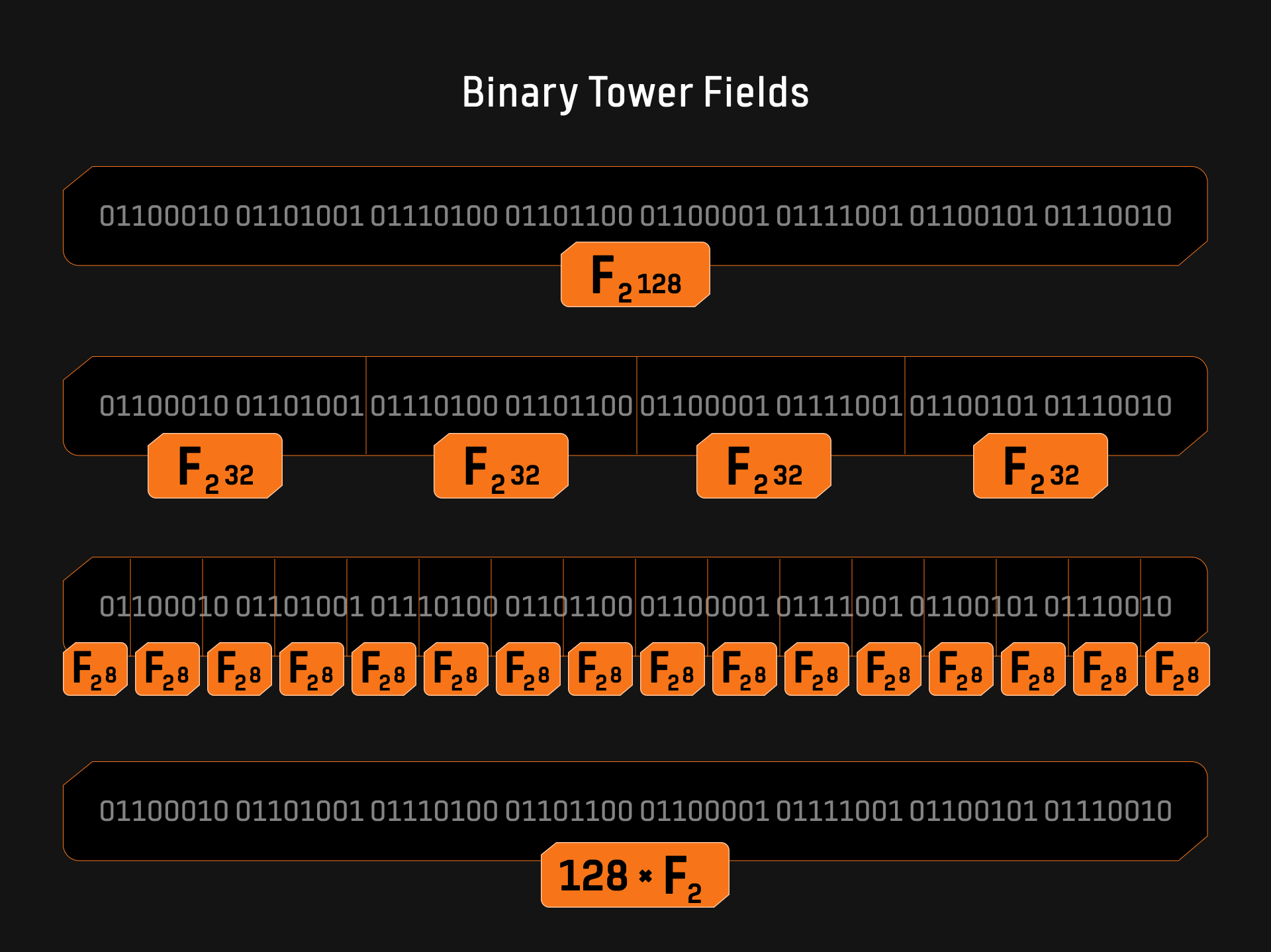
As shown in Figure 1, a 128-bit string can be interpreted in multiple ways within the context of a binary field. It can be viewed as a unique element in the 128-bit binary field, or it can be parsed as two 64-bit tower field elements, four 32-bit tower field elements, sixteen 8-bit tower field elements, or 128 elements of $\mathbb{F}_2$ . This flexibility in representation incurs no computational overhead, as it is merely a typecast of the bit string. This is a very interesting and useful property, as smaller field elements can be packed into larger field elements without additional computational cost. The Binius protocol leverages this property to enhance computational efficiency. Furthermore, the paper On Efficient Inversion in Tower Fields of Characteristic Two explores the computational complexity of multiplication, squaring, and inversion in $n$-bit tower binary fields (decomposable into $m$-bit subfields).
| Operation | Multiplication | m-bit Subfield Complexity | Square | Inversion |
|---|---|---|---|---|
| Complexity | $O(n^{1.58})$ | $O(nm^{0.58})$ | $O(n \log n)$ | $O(n^{1.58})$ |
2.2 PIOP: Adapted HyperPlonk Product and Permutation Check — Suitable for Binary Fields
The PIOP design in the Binius protocol draws inspiration from HyperPlonk and incorporates a series of core checks to verify the correctness of polynomials and multivariate sets. These checks are essential for ensuring the integrity of computations within the proof system, especially when operating over binary fields. The key checks include:
- GateCheck: Ensures that the private witness $\omega$ and public input $x$ satisfy the circuit operation relation $C(x, \omega) = 0$, verifying the correct execution of the circuit.
- PermutationCheck: Verifies that the evaluation results of two multivariate polynomials $f$ and $g$ on the Boolean hypercube form a permutation relation $f(x) = f(\pi(x))$, ensuring consistency between polynomial variables.
- LookupCheck: Checks if the evaluation of a polynomial is within a given lookup table, i.e., $f(B_\mu) \subseteq T(B_\mu)$, ensuring that certain values fall within a specified range.
- MultisetCheck: Confirms whether two multivariate sets are equal, i.e., ${(x_{1,i},x_{2,i})}{i \in H} = {(y{1,i},y_{2,i})}_{i \in H}$, ensuring consistency between different sets.
- ProductCheck: Ensures that the evaluation of a rational polynomial on the Boolean hypercube equals a declared value, i.e., $\prod_{x \in H_\mu} f(x) = s$, confirming the correctness of the polynomial product.
- ZeroCheck: Verifies whether a multivariate polynomial evaluates to zero at any point on the Boolean hypercube, i.e., $\prod_{x \in H_\mu} f(x) = 0$ for all $x \in B_\mu$, ensuring proper distribution of zeros in the polynomial.
- SumCheck: Confirms whether the sum of the evaluations of a multivariate polynomial equals the declared value, i.e., $\sum_{x \in H_\mu} f(x) = s$. By reducing the evaluation of multivariate polynomials to univariate polynomial evaluation, it lowers the verifier’s computational complexity. SumCheck also allows for batching, which constructs linear combinations using random numbers to batch-process multiple instances.
- BatchCheck: An extension of SumCheck, it verifies the correctness of multiple multivariate polynomial evaluations, increasing protocol efficiency.
While Binius and HyperPlonk share several similarities in their protocol designs, Binius introduces the following key improvements:
- ProductCheck Optimization: In HyperPlonk, ProductCheck requires the denominator $U$ to be non-zero across the entire hypercube, and that the product matches a specific value. Binius simplifies this check by setting the product value to 1, reducing the overall computational complexity.
- Handling of Zero-Division Issues: HyperPlonk does not effectively address zero-division problems, making it challenging to guarantee that $U$ remains non-zero over the hypercube. Binius resolves this by handling zero-division scenarios appropriately, enabling ProductCheck to function even when the denominator is zero, allowing for extensions to arbitrary product values.
- Cross-Column PermutationCheck: HyperPlonk lacks support for cross-column permutation checks. Binius addresses this limitation by introducing support for cross-column PermutationCheck, enabling the protocol to manage more complex polynomial permutations across multiple columns.
Thus, Binius enhances the flexibility and efficiency of the protocol by improving the existing PIOP SumCheck mechanism, particularly by providing stronger functionality for verifying more complex multivariate polynomials. These improvements not only address the limitations of HyperPlonk but also lay the foundation for future proof systems based on binary fields.
2.3 PIOP: A New Multilinear Shift Argument—Applicable to Boolean Hypercube
In the Binius protocol, the manipulation and construction of virtual polynomials play a crucial role in enabling efficient polynomial handling. Two main techniques are employed for these operations:
- Packing :The packing method optimizes the handling of smaller elements by grouping them together in a larger domain. Specifically, elements adjacent in lexicographic order are packed into larger blocks, typically of size $2^\kappa$. By leveraging Multilinear Extension (MLE), the packed elements are transformed into a new virtual polynomial, which can then be evaluated and processed efficiently. This method enhances the performance of operations on the Boolean hypercube by restructuring the function $t$ into a computationally efficient form.
- Shift Operator : The shift operator rearranges elements within a block by cyclically shifting them based on a given offset $o$. This shift applies to blocks of size $2^b$, ensuring that all elements in a block are shifted uniformly according to the predefined offset. This operator is particularly useful when dealing with virtual polynomials in high-dimensional spaces, as its complexity increases linearly with the block size, making it an ideal technique for large datasets or complex Boolean hypercube computations.
2.4 PIOP: An Adapted Lasso Lookup Argument—Applicable to Binary Fields
The Lasso protocol in Binius offers a highly efficient method for proving that elements in a vector $a \in \mathbb{F}^m$ are contained within a predefined table $t \in \mathbb{F}^n$ . This lookup argument introduces the concept of “Lookup Singularity” and is well-suited for multilinear polynomial commitment schemes. The efficiency of Lasso is highlighted in two major aspects:
- Proof Efficiency : When conducting $m$ lookups in a table of size $n$, the prover only needs to commit to $m + n$ small field elements, with the field size drawn from the set ${0, \dots, m}$. In cryptographic schemes that rely on exponentiation, the prover’s cost is $O(m + n)$ group operations (e.g., elliptic curve point additions). This efficiency comes in addition to the cost of verifying whether a multilinear polynomial evaluated on the Boolean hypercube matches a table element.
- No Commitment to Large Tables : If the table $t$ is structured, Lasso does not require a direct commitment to the table, making it possible to handle very large tables (e.g., $2^{128}$ or more). The prover’s runtime depends solely on the specific entries accessed in the table. For any integer parameter $c > 1$, the main cost involves proof size, which grows as $3 \cdot c \cdot m + c \cdot n^{1/c}$ committed field elements. These elements are also small, drawn from the set ${0, \dots, \max{m, n^{1/c}, q} - 1}$, where $q$ is the largest value in the vector $a$.
The Lasso protocol consists of three core components:
- Virtual Polynomial Abstraction of Large Tables : The Lasso protocol combines virtual polynomials to enable efficient lookups and operations on large tables, ensuring scalability without performance degradation.
- Small Table Lookup : At the heart of Lasso lies the small table lookup, which verifies whether a virtual polynomial evaluated on a Boolean hypercube is a subset of another virtual polynomial’s evaluations. This process is akin to offline memory detection and boils down to a multiset detection task.
- Multiset Check : The protocol also incorporates a virtual mechanism to perform multiset checks, ensuring that two sets of elements either match or fulfill predefined conditions.
The Binius protocol adapts Lasso for binary field operations, assuming the current field is a prime field of large characteristic (much larger than the length of the column being looked up). Binius introduces a multiplicative version of the Lasso protocol, requiring the prover and verifier to increment the protocol’s “memory counter” operation not simply by adding 1 but by incrementing using a multiplicative generator within the binary field. However, this multiplicative adaptation introduces additional complexity: unlike an additive increment, the multiplicative generator does not increment in all cases, instead having a single orbit at 0, which may present an attack vector. To mitigate this potential attack, the prover must commit to a read counter vector that is non-zero everywhere to ensure protocol security.
2.5 PCS: Adapted Brakedown PCS—Applicable to Small Fields
The core idea behind constructing the Binius PCS (Polynomial Commitment Scheme) is packing. The Binius paper presents two Brakedown PCS schemes based on binary fields: one instantiated using concatenated codes, and another using block-level encoding, which supports the standalone use of Reed-Solomon codes. The second Brakedown PCS scheme simplifies the proof and verification process, though it produces a slightly larger proof size than the first one; however, this trade-off is worthwhile due to the simplification and implementation benefits it offers.
The Binius polynomial commitment primarily utilizes small-field polynomial commitment with evaluations in an extended field, small-field universal construction, and block-level encoding with Reed-Solomon code techniques.
Small-Field Polynomial Commitment with Extended Field Evaluation In the Binius protocol, polynomial commitments are performed over a small field $K$, with evaluations taking place in an extended field $L/K$. This technique ensures that a multilinear polynomial $t(X_0, \dots, X_{\ell-1})$ belongs to the domain $K[X_0, \dots, X_{\ell-1}]$, while the evaluation points are in the larger field $L$. This commitment structure enables efficient queries within the extended field, balancing security and computational efficiency.
Small-Field Universal Construction This construction defines key parameters like the field $K$, its dimension $\ell$, and the associated linear block code $C$, while ensuring that the extended field $L$ is large enough for secure evaluations. By leveraging properties of the extended field, Binius achieves robust commitments through linear block codes, maintaining a balance between computational efficiency and security.
Block-Level Encoding with Reed-Solomon Codes For polynomials defined over small fields like $\mathbb{F}2$ , the Binius protocol employs block-level encoding using Reed-Solomon codes. This scheme allows efficient commitment of small-field polynomials by encoding them row-by-row into larger fields (such as $\mathbb{F}{2^{16}}$ ), utilizing the efficiency and maximum distance separable properties of Reed-Solomon codes. After encoding, these rows are committed using a Merkle tree, which simplifies the operational complexity of small-field polynomial commitments. This approach allows for the efficient handling of polynomials in small fields without the computational burden usually associated with larger fields.
3. Binius Optimizations
To further improve performance, Binius incorporates four major optimizations:
- GKR-based PIOP : The GKR (Goldreich-Kalai-Rothblum) protocol is used to replace the Lasso Lookup algorithm in binary field multiplication, significantly reducing the overhead in the commitment process.
- ZeroCheck PIOP Optimization : This optimization addresses the balance between the Prover and Verifier’s computational costs, making the ZeroCheck operation more efficient by distributing workload more effectively.
- Sumcheck PIOP Optimization : By optimizing the small-field Sumcheck process, Binius reduces the overall computational burden when operating over small fields.
- PCS Optimization : Using FRI-Binius (Fast Reed-Solomon Interactive Oracle Proofs of Proximity) optimization, Binius reduces proof size and enhances protocol performance, improving overall efficiency in both proof generation and verification.
3.1 GKR-based PIOP: Binary Field Multiplication Using GKR
In the original Binius protocol, binary field multiplication is handled through a lookup-based scheme, which ties multiplication to linear addition operations based on the number of limbs in a word. While this method optimizes binary multiplication to an extent, it still introduces auxiliary commitments linearly related to the number of limbs. By adopting a GKR-based approach, the Binius protocol can significantly reduce the number of required commitments, leading to further efficiency in binary field multiplication operations.
The core idea of the GKR (Goldwasser-Kalai-Rothblum) protocol is to achieve agreement between the Prover (P) and Verifier (V) over a layered arithmetic circuit on a finite field $\mathbb{F}$ . Each node in this circuit has two inputs for computing the required function. To reduce the Verifier’s computational complexity, the protocol employs the SumCheck protocol, which progressively reduces claims about the circuit’s output gate values to lower-layer gate values, eventually simplifying the claims to statements about the inputs. This way, the Verifier only needs to verify the correctness of the circuit inputs.
The GKR-based integer multiplication algorithm in Binius transforms the check of whether two 32-bit integers $ A $ and $ B $ satisfy $ A \cdot B \overset{?}{=} C $ into verifying whether $ (g^A)^B \overset{?}{=} g^C $ holds in $ \mathbb{F}_{2^{64}}^*$ . This transformation, combined with the GKR protocol, significantly reduces the overhead associated with polynomial commitments. Compared to the previous Binius lookup-based scheme, the GKR-based multiplication approach requires only one auxiliary commitment and reduces the cost of SumChecks, making the algorithm more efficient, especially in cases where SumChecks are more economical than additional commitments. This method is becoming a promising solution for minimizing binary field polynomial commitment costs as Binius optimizations progress.
3.2 ZeroCheck PIOP Optimization: Balancing Computational Costs between Prover and Verifier
The paper Some Improvements for the PIOP for ZeroCheck proposes strategies to balance computational costs between the Prover (P) and Verifier (V), focusing on reducing data transmission and computational complexity. Below are key optimization techniques:
1. Reducing Prover’s Data Transmission
By transferring some of the computational burden to the Verifier, the Prover’s data transmission can be minimized. For instance, in round $ i $, the Prover sends $ v_{i+1}(X) $ for $ X = 0, \dots, d+1 $, and the Verifier checks whether $v_i = v_{i+1}(0) + v_{i+1}(1)$ holds.
Optimization: The Prover can avoid sending $ v_{i+1}(1) $, as the Verifier can compute it as $v_{i+1}(1) = v_i - v_{i+1}(0)$.
In the initial round, the Prover sends $ v_1(0) = v_1(1) = 0 $, eliminating some evaluation calculations, which reduces both computational and transmission costs to $d2^{n-1}C_\mathbb{F} + (d + 1)2^{n-1}C_\mathbb{G}$ .
2. Reducing the Number of Evaluation Points for the Prover
During round $ i $, the Prover must send $ v_{i+1}(X) $, calculated as $v_{i+1}(X) = \sum_{x \in H_{n-i-1}} \hat{\delta}_n(\alpha, (r, X, x)) C(r, X, x)$ .
Optimization: Instead, the Prover can send \(v_{i+1}'(X) = \sum_{x \in H_{n-i-1}} \hat{\delta}_n(\alpha_{i+1}, \dots, \alpha_{n-1}, x) C(r, X, x),\)
where $v_i(X) = v_i’(X) \cdot \hat{\delta}{i+1}((\alpha_0, \dots, \alpha_i), (r, X))$ . As the Verifier has access to $\alpha$ and $r$, the degree of $v_i’(X)$ is lower than that of $ v_i(X) $, reducing the required evaluation points. The inter-round check can then be simplified as $(1 - \alpha_i)v{i+1}’(0) + \alpha_i v_{i+1}’(1) = v_i’(X),$ thereby lowering data transmission needs and enhancing efficiency. With these improvements, the overall cost is approximately $2^{n-1}(d - 1)C_F + 2^{n-1}dC_G.$ For $d = 3$ , these optimizations yield a cost reduction by a factor of 5/3.
3. Algebraic Interpolation Optimization
For an honest Prover, the polynomial $ C(x_0, \dots, x_{n-1}) $ is zero on $ H_n $ and can be expressed as $C(x_0, \dots, x_{n-1}) = \sum_{i=0}^{n-1} x_i(x_i - 1) Q_i(x_0, \dots, x_{n-1})$. Where $ Q_i $ is computed through ordered polynomial division, starting from $ R_n = C $. Sequential division by $ x_i(x_i - 1) $ computes $ Q_i $ and $ R_i $, with $ R_0 $ representing the multilinear extension of $ C $ on $ H_n $, assumed to be zero.
Analyzing the Degrees of $ Q_i $. For $ j > i $, $ Q_j $ retains the same degree in $ x_i $ as $ C $. For $ j = i $, the degree is reduced by 2, and for $ j < i $, the degree is at most 1. Given a vector $ r = (r_0, \dots, r_i) $, $ Q_j(r, X) $ is multilinear for all $ j \leq i $. Moreover, $ Q_i(r, X) = \sum_{j=0}^{i} r_j(r_j - 1) Q_j(r, X) $ is the unique multilinear polynomial matching $ C(r, X) $ on $ H_{n-i} $. For any $ X $ and $ x \in H_{n-i-1} $, it can be represented as $C(r, X, x) - Q_i(r, X, x) = X(X - 1) Q_{i+1}(r, X, x).$ Thus, during each round of the protocol, a new $ Q $ is introduced, and its evaluation can be derived from $ C $ and the previous $ Q $, allowing for interpolation optimization.
3.3 Sumcheck PIOP Optimization: Small-Field Sumcheck Protocol
In the STARKs protocol implemented by Binius, the primary bottleneck for the prover is often the sum-check protocol rather than the Polynomial Commitment Scheme (PCS), due to the low commitment cost.
In 2024, Ingonyama proposed improvements for small-field-based Sumcheck protocols, focusing on Algorithms 3 and 4. These improvements were implemented and made publicly available here. Algorithm 4 incorporates the Karatsuba algorithm into Algorithm 3, reducing the number of extension field multiplications in exchange for more base field multiplications. This approach is more efficient when extension field multiplications are more expensive than base field ones.
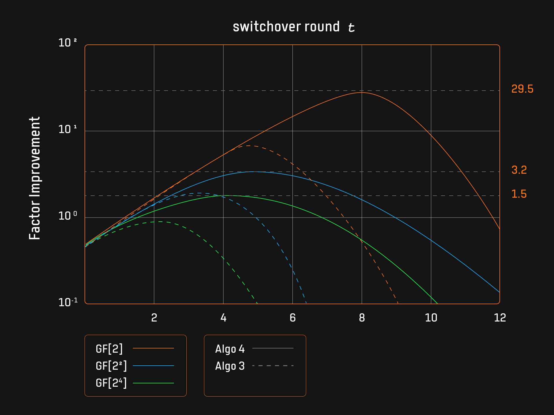
1. Impact of Switchover Rounds and Improvement Factors The small-field Sumcheck protocol’s optimization hinges on selecting the optimal switchover round $ t $, which marks when the protocol reverts from the optimized version to the naive algorithm. Experiments indicate that the improvement factor peaks at the optimal switchover point and then follows a parabolic trend. When this point is exceeded, efficiency diminishes because the ratio between base field and extension field multiplications is greater in smaller fields, necessitating a timely reversion to the naive algorithm.
For certain applications, like the Cubic Sumcheck ($ d = 3 $), the small-field Sumcheck protocol delivers an order-of-magnitude improvement over the naive approach. For instance, in the base field $ GF[2] $, Algorithm 4 outperforms the naive algorithm by nearly 30 times.
2. Impact of Base Field Size on Performance Smaller base fields (e.g., $ GF[2] $) significantly enhance the efficiency of the optimized algorithm due to the larger disparity between the costs of extension field and base field multiplications. This leads to a more substantial improvement factor for the optimized algorithm.
3. Optimization Gains from the Karatsuba Algorithm The Karatsuba algorithm plays a crucial role in improving the performance of the small-field Sumcheck protocol. For a base field of $ GF[2] $, Algorithm 4 achieves peak improvement factors of 6 for Algorithm 3 and 30 for Algorithm 4, indicating that Algorithm 4 is five times more efficient than Algorithm 3. The Karatsuba algorithm enhances runtime efficiency and optimizes the switchover point for both algorithms, with optimal points at $ t = 5 $ for Algorithm 3 and $ t = 8 $ for Algorithm 4.
4. Memory Efficiency Improvements The small-field Sumcheck protocol also boosts memory efficiency. Algorithm 4 requires $O(d \cdot t)$ memory, while Algorithm 3 needs $ O(2^d \cdot t) $ memory. For $t = 8$ , Algorithm 4 uses just 0.26 MB of memory, compared to the 67 MB required by Algorithm 3. This makes Algorithm 4 particularly suitable for memory-constrained environments, such as client-side proving with limited resources.
3.4 PCS Optimization: FRI-Binius Reducing Binius Proof Size
One of the main challenges of the Binius protocol is its relatively large proof size, which scales with the square root of the witness size at $O(\sqrt{N})$ . This square-root scaling limits its competitiveness when compared to systems offering more succinct proofs. In contrast, polylogarithmic proof sizes, as achieved by advanced systems like Plonky3 through techniques such as FRI, are essential for ensuring truly “succinct” verifiers. The FRI-Binius optimization aims to reduce Binius’ proof size and improve its overall performance in comparison to more efficient systems.
The paper Polylogarithmic Proofs for Multilinears over Binary Towers, referred to as FRI-Binius, introduces a novel binary-field-based FRI (Fast Reed-Solomon Interactive Oracle Proof of Proximity) folding mechanism with four key innovations:
- Flattened Polynomials: Transforms the initial multilinear polynomial into a Low Code Height (LCH) polynomial basis for optimized computation.
- Subspace Vanishing Polynomials: Utilizes these polynomials in conjunction with an additive NTT (Number Theoretic Transform) to enable FFT-like decomposition, optimizing operations over the coefficient field.
- Algebraic Basis Packing: Facilitates efficient data packing, minimizing the protocol’s overhead related to embedding.
- Ring-Switching SumCheck: A new SumCheck optimization using ring-switching techniques to further enhance performance.
Core Process of FRI-Binius Multilinear Polynomial Commitment Scheme (PCS)
The FRI-Binius protocol optimizes binary-field multilinear polynomial commitment schemes (PCS) by transforming the initial multilinear polynomial, defined over the binary field $ \mathbb{F}_2$ , into a multilinear polynomial over a larger field $ K $.
- Commitment Phase The commitment phase transforms an $\ell$-variable multilinear polynomial (over $\mathbb{F}2$ ) into a commitment for a packed $\ell’$-variable multilinear polynomial (over $\mathbb{F}{2^{128}}$ ). This process reduces the number of coefficients by a factor of 128, allowing for more efficient proof generation.
- Evaluation Phase In this phase, the prover and verifier execute $\ell’$ rounds of a cross-ring switching SumCheck protocol combined with FRI interactive oracle proofs of proximity (IOPP). Key details include:
- FRI Opening Proofs: These make up the majority of the proof size and are handled similarly to standard FRI proofs over large fields.
- Prover’s SumCheck Cost: Comparable to the cost of executing SumCheck in a large field.
- Prover’s FRI Cost: Matches the standard FRI costs seen in large-field implementations.
- Verifier’s Operations: The verifier receives 128 elements from $\mathbb{F}_{2^{128}}$ and performs 128 additional multiplications, allowing for efficient verification.
Benefits of FRI-Binius
By applying this method, Binius is able to reduce its proof size by an order of magnitude, bringing it closer to the performance of state-of-the-art cryptographic systems, while remaining compatible with binary fields. The FRI folding method, optimized for binary fields, combined with algebraic packing and SumCheck optimizations, helps Binius generate smaller proofs without compromising verification efficiency.
This transformation marks a significant step toward improving proof size in Binius, ensuring that it becomes more competitive with other cutting-edge systems, particularly those focused on polylogarithmic proof sizes.
| Total Data Size | Coeff. Size | Packing Factor | Binius Proof Size (MiB) | FRI-Binius Proof Size (MiB) |
|---|---|---|---|---|
| 512MB (2^32 bits) | 6 | 0 | 2.7 | 0.55 |
| 3 | 2 | 5.4 | 0.95 | |
| 0 | 4 | 10.8 | 3.51 | |
| 8.192 GiB (2^36 bits) | 6 | 0 | 10.8 | 0.74 |
| 3 | 2 | 21.6 | 1.28 | |
| 0 | 5 | 59.1 | 4.58 |
| Scheme | Coeff. Bits | Current Size (MiB) | Optimized Size (MiB) | Commit + Prove Time (s) |
|---|---|---|---|---|
| Plonky3 FRI | 31 | 1.1 | 0.31 | 9.55 |
| FRI-Binius | 1 | 0.84 | 0.16 | 0.91 |
| FRI-Binius | 8 | 1.09 | 0.20 | 7.6 |
| FRI-Binius | 32 | 1.29 | 0.24 | 28.9 |
4. Conclusion
The entire value proposition of Binius lies in its ability to use the smallest power-of-two field size for witnesses, selecting the field size as needed. Binius is a co-design scheme for “hardware, software, and FPGA-accelerated Sumcheck protocols,” enabling fast proofs with very low memory usage.
Proof systems like Halo2 and Plonky3 involve four key computationally intensive steps: generating witness data, committing to the witness data, performing a vanishing argument, and generating the opening proof.
For example, with the Keccak hash function in Plonky3 and the Grøstl hash function in Binius, the computational distribution for these four key steps is illustrated in Figure 3.

This comparison shows that Binius has essentially eliminated the prover’s commitment bottleneck. The new bottleneck is the Sumcheck protocol, where issues such as numerous polynomial evaluations and field multiplications can be efficiently addressed with specialized hardware.
The FRI-Binius scheme, a variant of FRI, offers a highly attractive option by removing embedding overhead from the field proof layer without causing a significant cost increase in the aggregated proof layer.
Currently, the Irreducible team is developing its recursive layer and has announced a partnership with the Polygon team to build a Binius-based zkVM; the Jolt zkVM is transitioning from Lasso to Binius to enhance its recursive performance; and the Ingonyama team is implementing an FPGA version of Binius.
References
- 2024.04 Binius Succinct Arguments over Towers of Binary Fields
- 2024.07 Fri-Binius Polylogarithmic Proofs for Multilinears over Binary Towers
- 2024.08 Integer Multiplication in Binius: GKR-based approach
- 2024.06 zkStudyClub - FRI-Binius: Polylogarithmic Proofs for Multilinears over Binary Towers
- 2024.04 ZK11: Binius: a Hardware-Optimized SNARK - Jim Posen
- 2023.12 Episode 303: A Dive into Binius with Ulvetanna
- 2024.09 Designing high-performance zkVMs
- 2024.07 Sumcheck and Open-Binius
- 2024.04 Binius: highly efficient proofs over binary fields
- 2023.12 SNARKs on binary fields: Binius - Part 1
- 2024.06 SNARKs on binary fields: Binius - Part 2
- 2022.10 HyperPlonk, a zk-proof system for ZKEVMs